In this short note, we will try to improve readers’ intuition on the duration and convexity of bonds.
To talk about convexity, we first need to know what the duration is.
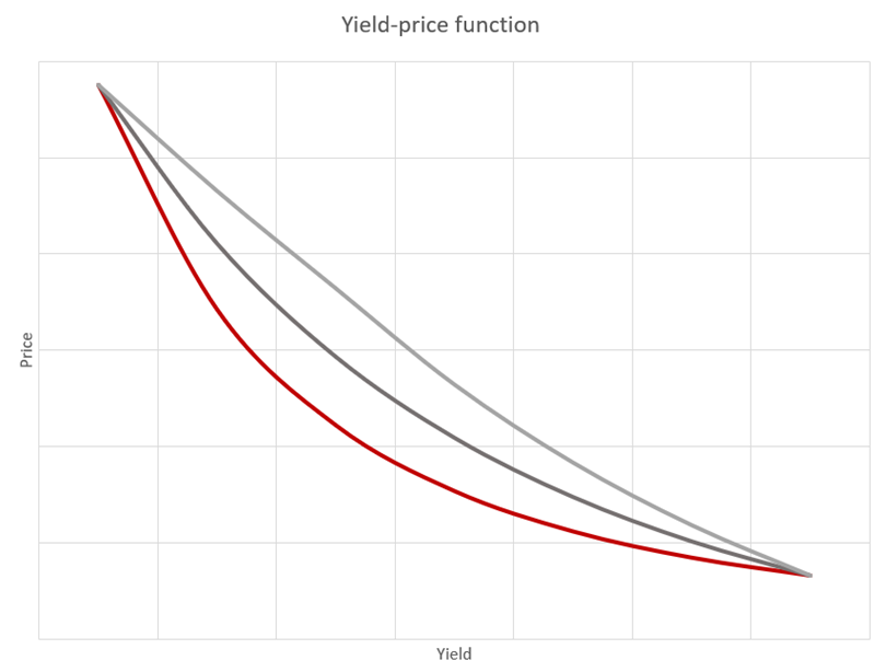
Below is the graph that represents the connection between a bond’s yield and price.
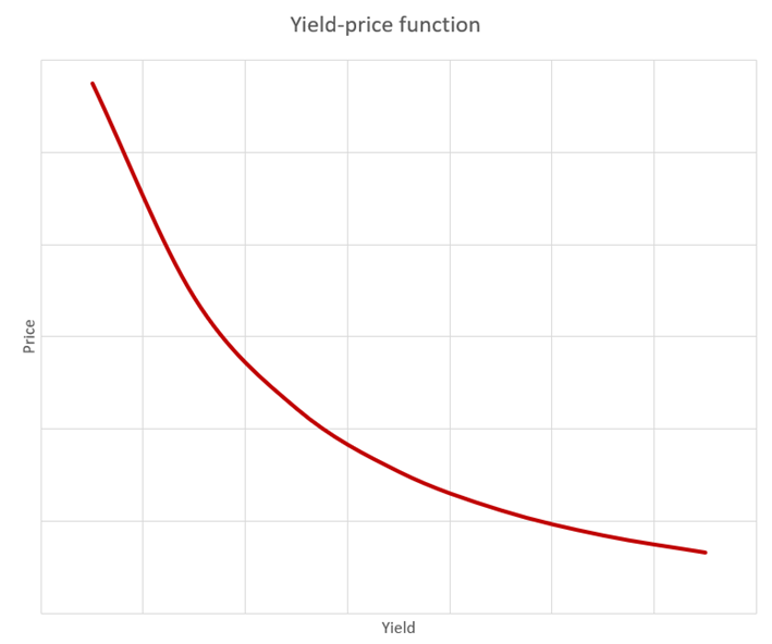
Just by observing, the yield-price function graph gives us a few interesting takeaways. In Mathematics it is said that function is strictly decreasing which translates into „the yield is falling if and only if the price is rising and the yield is rising if and only if the price is falling“. We have not got far, but stay with us, now comes the fun part.
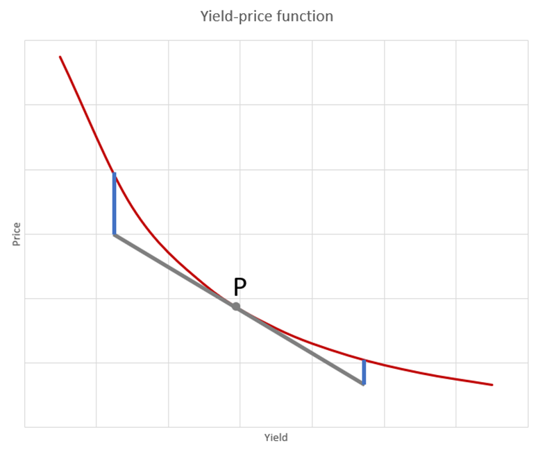
From the point of the Mathematical Analysis, you would want to know what the derivative of the function is. So, let us pick a point on the x-axis, call it P, and find the derivative in that point. The derivative is the slope of a line that is tangent to the function at that point, as the following picture shows.
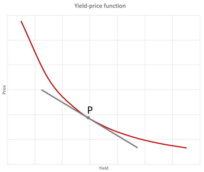
The derivative that was just calculated is sometimes known as the modified duration of a bond. Again, just by observing the graph above, we can see that the duration tells us how much we can expect the price to move after a movement in the yield. We can conclude that a „small“ duration means a movement in yield results in a relatively small movement in the price.
Simple logical deduction leads us to the following conclusion: a „big“ duration means a movement in the yield results in a relatively big movement in the price.
In other words, an investor who is looking for a smaller amount of volatility should be investing in bonds with a smaller duration, ceteris paribus.
Alongside the Mathematical Analysis point of view, there is also a Probabilistic approach which is a bit different.
Imagine a seesaw. One point of a seesaw is the issuance of a bond, and the other end is the maturity date. Put a weight on the maturity date that represents the bond’s principal in sum with the last coupon. The issuance end of the seesaw remains empty. The rest of the seesaw is divided into equal parts (the number of parts is the number of cash flows from a bond), with a weight that represents one coupon, as the next picture presents.
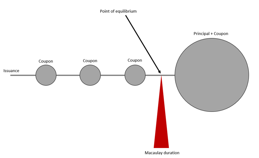
The equilibrium point of the seesaw is called Macaulay duration and is close to the modified duration. Macaulay duration we can interpret as the average time that needs to pass to return money invested in a bond.
From now on, we will not differentiate between these two durations, and we will call them just duration.
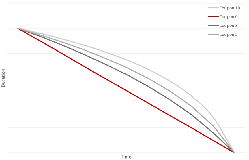
From the last remark, we conclude that the duration on zero coupon bonds decreases linearly from [years to maturity] towards zero. Bonds that have coupons strictly greater than 0 don’t have a linear change in duration with time, but during the first period of time duration slowly decreases, and toward maturity has a stronger decrease (because the most weight is in the last period), which is presented on the following graph.
Convexity
With a better understanding of duration, we can now move to convexity. Let’s examine the next graph.
The last graph motivates the definition of the curvature of a curve. Curvature is a measure in Mathematics that says how much a curve is curved, for which we would like that:
- a line has a zero curvature.
- a big circle has a smaller curvature than a small circle (because a bigger circle is locally closer to the line).
- a circle has constant curvature.
Somewhere in a theory known as Differential Geometry, mathematicians did find that measure. It is expressed through a derivative of a derivative that is sometimes called a second derivative.
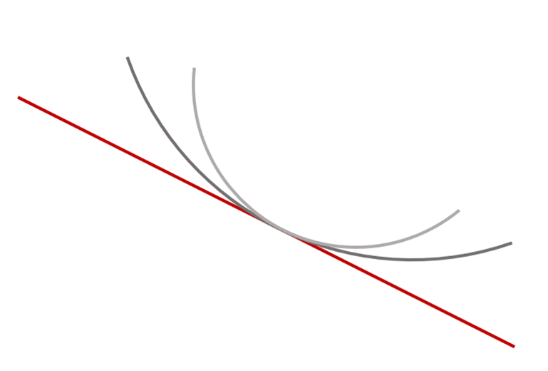
We are going back to our yield-price function, and we want to know how much it is curved. The following graph shows yield-price functions with different curvatures.
The curvature of a yield-price function we call the convexity of a bond. We are trying to avoid mathematical language, but a reader should be aware that convexity is close to the second derivative of a yield-price function (or equivalently, with convexity, we measure how much duration is sensitive on movements). The last graph shows us the importance of convexity. With smaller convexity on a bond, the yield-price function is closer to a line, and the approximation of a future price calculated with a duration is closer to the actual price of a bond after the movement.
We can conclude that duration gives us intuition on how much a price will move after a relatively small movement in yield, and convexity gives us information on how much approximation by duration will be precise.
For example, the Italian 10-year bond, which can be found under ticker ITALY 5 3/8 06/15/33, currently has a price of 93.494 and a yield of 6.285%. The coupon is 5.375. If a yield falls by 3% (on a 3.285%) the price moves to 117.11, which is a 25.26% increase in price. On the other side, if a yield rises by 3% (on a 9.285%), the price moves to 75.464, a decrease in the price of 19.3%. As we can see, the price doesn’t change linearly due to convexity. The duration for this bond is 7.395, which is very high, due to which a price has large movements (over 20%) after just a 3% movement in the yield.
To sum up, if we want the small volatility of a bond, then we need to find a bond with a small duration and a small convexity.
In that regard, bonds on the long end with small yields are especially dangerous because they have a long duration due to long maturity, so the risk-reward is very unfavourable. For a small gain (carry of a small yield), you take a big risk (capital loss) if yields move to slightly higher levels.
The importance of duration and convexity comes from the Fundamental theorem for curves that says that the whole behavior of the yield-price function is explained with these two measures. That is the reason why we always mention duration and convexity and we hope that we managed to bring closer this topic to you.