In this series of blog posts, we will delve into the intricacies of the realized volatility across a range of financial instruments. Most notably, we will show how several stylized facts persist across asset classes and hold through different market regimes.

When examining the price action of a given instrument, realized volatility focuses on the amplitudes of moves rather than their direction. A practical challenge is that realized volatility is a latent quantity: it cannot be observed instantaneously but is inferred from price movements over a specified time period. In this series, we compute realized volatility as the square root of the variance of daily close‑to‑close logarithmic returns, assuming zero drift, and we annualize the result. We also acknowledge the downward bias introduced by Jensen’s inequality.

Market participants often rationalize price action ex post, justifying price action by finding a suitable rationale. Moves are attributed to news or announcements released over the relevant window. Because different types of news affect asset classes to varying degrees, one might not expect common patterns. Nevertheless, statistical analysis shows that the realized volatility of many instruments exhibits similar behaviours, suggesting a degree of generalizability. It is important to note that it can be difficult to discern which stylized fact dominates at a given moment, or how to reconcile cases where two stylized facts point to opposite conclusions regarding the future movement of realized volatility.

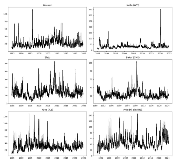
The first stylized fact we explore is the horizontal (time) dependence of volatility. It shows how realized volatility isn’t constant through time but has a tendency to revert to its historical mean. That reversion happens gradually, such that periods of high/low volatility are typically followed by similar values, a phenomenon known as volatility clustering. This aligns with the observation that realized volatility, unlike raw returns, displays meaningful autocorrelation, also known as saying that volatility is a long-memory process. Below is a chart of one‑month realized volatility, in percentage points, for a selected set of commodities.

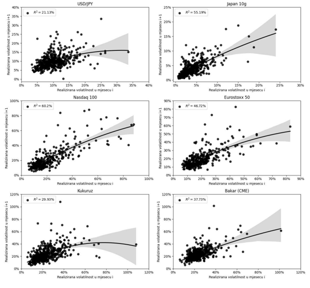
We then show that clustering does not hinge on the asset class. The same behavior appears across equities (indices and single names), commodities, currencies, and fixed income. As the commodity example above illustrates, a simple takeaway is that, in many cases, the best estimate of near‑term realized volatility is the level observed in the recent past. We show that in the following graph, where the y-axis shows how realized volatility in month t+1 depends on the realized volatility in month t. Each panel also reports the coefficient of determination (R²) from a second‑degree polynomial fit.

We conclude this first post after introducing realized volatility and exploring its temporal dependence and clustering. In the next instalment, we will examine autocorrelations of returns, the velocity at which realized volatility converges toward its long‑term mean, and selected moments of the return distribution, including skewness and kurtosis.